IGEE

Articles
- Page Path
- HOME > IGEE Proc > Forthcoming articles > Article
-
Article
Environmental Inequality and Socioeconomic Vulnerability: A Meta-Analysis and Exploratory GIS-Based Spatial Analysis of Seoul - Seoyoung Park1*, Minseo Kim2, Dayoung Lee1, Seohyun Lee2, Sohye Lee2
-
DOI: https://doi.org/10.69841/igee.2026.023
Published online: October 22, 2026
1Department of Chinese Language and Literature, Yonsei University, Sinchon, Korea
2Department of Nursing, Yonsei University, Sinchon, Korea
- *Corresponding author: Seoyoung Park, E-mail: psy7973@gmail.com
• Received: February 4, 2026 • Revised: June 12, 2026 • Accepted: October 14, 2026
© 2026 by the authors.
Submitted for possible open-access publication under the terms and conditions of the Creative Commons Attribution (CC BY) license (http://creativecommons.org/licenses/by/4.0/).
- 33 Views
- 3 Download

Abstract
-
Background
- Environmental inequality refers to the unequal distribution of environmental risks and benefits across social groups and geographic areas. Previous studies have reported associations between various environmental indicators and socioeconomic factors; however, substantial heterogeneity across studies has limited the ability to draw generalized conclusions. Therefore, this study aimed to synthesize the overall pattern of association between environmental disadvantage and socioeconomic vulnerability reported in previous empirical studies, explore how related spatial patterns are manifested within Seoul, and consider their implications for environmental justice screening and ESG-informed urban environmental governance.
-
Methods
- Following the PRISMA guidelines, a systematic review of domestic and international literature was conducted, and a random-effects meta-analysis was performed on ten empirical studies. Effect sizes were based on reported correlation coefficients (r), which were transformed using Fisher’s z transformation, pooled, and subsequently converted back to correlation coefficients. In addition, an exploratory area-level GIS analysis was conducted across 426 administrative dongs (neighborhood-level administrative units) in Seoul, South Korea. Potential environmental burden was represented by the proportion of land area located within a 300-m proximity zone surrounding environmental infrastructure facilities, while housing vulnerability was represented by the proportion of publicly supported housing. The association between these proxy indicators was examined using correlation analysis, and spatial clustering of the environmental facility proximity indicator was assessed using Global Moran’s I and Local Indicators of Spatial Association (LISA).
-
Results
- The meta-analysis yielded a positive pooled association between environmental disadvantage and socioeconomic vulnerability (r = 0.316, 95% CI: 0.183–0.438), although substantial between-study heterogeneity indicated considerable variation across research contexts. The GIS analysis of Seoul identified a weak positive area-level association between the 300-m environmental facility proximity indicator and the publicly supported housing ratio (r = 0.187, R² = 0.035). Furthermore, the Global Moran’s I analysis showed statistically significant positive spatial autocorrelation in the environmental facility proximity indicator (I = 0.216, z = 7.790, pseudo p = 0.001; 999 permutations). A 500-m sensitivity analysis produced similar directional results.
-
Conclusions
- This study quantitatively synthesized evidence suggesting an overall positive relationship between environmental inequality and socioeconomic vulnerability. The Seoul case study further provided exploratory evidence of a weak positive association between environmental facility proximity and the proportion of publicly supported housing, as well as the presence of localized spatial clustering patterns. However, given the limited number of included studies, the substantial heterogeneity among them, and the use of proxy measures for both environmental burden and housing vulnerability in the GIS analysis, the findings should be interpreted as preliminary evidence rather than definitive causal conclusions. Accordingly, the Seoul analysis should be interpreted as a screening-oriented exploratory assessment that may help identify candidate areas for more detailed environmental and socioeconomic investigation, rather than as a stand-alone basis for designating environmentally unjust areas or determining direct policy intervention.
- Environmental inequality refers to the uneven distribution of environmental risks and benefits across social groups and geographic areas. In urban environments, living conditions such as air pollution, noise exposure, flood risk, access to green spaces, and proximity to environmental infrastructure often vary substantially between neighborhoods. These disparities carry important policy implications when combined with socioeconomic vulnerability. Populations with limited residential mobility, restricted access to environmental information, lower capacity to file complaints, or fewer resources to mitigate environmental burdens may face greater difficulty avoiding or reducing the impacts of environmental hazards.
- Research on environmental justice has consistently highlighted the close relationship between environmental risks and socioeconomic conditions. Mohai et al. (2009) identified the disproportionate concentration of environmental hazards among specific social groups and regions as a central issue in environmental justice research. Hajat et al. (2015) reviewed socioeconomic disparities in air pollution exposure and reported that low-income and socially vulnerable populations are often exposed to higher levels of environmental risk. Similarly, Wolch et al. (2014) emphasized that access to urban green spaces and parks is strongly associated with health outcomes, quality of life, and environmental justice, while also noting that the distribution of green infrastructure may vary according to socioeconomic conditions. Together, these studies suggest that environmental inequality is not limited to a single environmental factor but rather reflects a complex interaction between urban environmental conditions and socioeconomic vulnerability.
- Environmental justice is a multidimensional concept that encompasses not only the distribution of environmental burdens and benefits but also issues of recognition and participation (Schlosberg, 2007). The present study is primarily situated within the distributive dimension of environmental justice, which concerns how environmental burdens and benefits are distributed across social groups and geographic areas. Accordingly, this study does not attempt to evaluate environmental justice in its entirety. Rather, it examines whether indicators of potential environmental disadvantage tend to coincide with indicators of socioeconomic vulnerability across previous empirical studies and within urban space.
- Despite growing evidence, previous studies differ considerably in terms of environmental indicators, study regions, spatial units, and socioeconomic measures, making it difficult to identify a general pattern across findings. Associations between socioeconomic vulnerability and environmentally disadvantaged conditions have been reported in diverse domains, including air pollution, green-space accessibility, flood risk, hazardous substance exposure, and transportation accessibility(Park & Song, 2014; Chakraborty & Basu, 2021; Myeong, 2017; Padilla et al., 2014; Tyrrell et al., 2013; Verbeek, 2019; Han et al., 2014; Seo & Jun, 2011; Seo & Han, 2019; Næss et al., 2007). However, the magnitude and consistency of these relationships vary substantially across studies. Therefore, there is a need to quantitatively synthesize existing evidence to examine the overall direction and magnitude of association between environmental disadvantage and socioeconomic vulnerability across heterogeneous research contexts. Meta-analysis provides a useful approach for integrating effect sizes reported in different studies and identifying common patterns observed across diverse research contexts.
- However, while meta-analysis can reveal average associations reported in previous studies, it cannot directly illustrate how environmental burdens and social vulnerability are spatially distributed within a specific city. Urban policy requires not only an understanding of overall average relationships but also an examination of how environmental facility proximity and social vulnerability indicators are spatially distributed and associated within urban space. Geographic Information System (GIS)-based spatial analysis can complement meta-analysis by examining the relationships, distributions, and spatial clustering of environmental and social vulnerability indicators at detailed spatial scales such as administrative neighborhoods.
- In the Seoul GIS analysis, environmental facility proximity and the proportion of publicly supported housing were employed as proxy indicators of potential environmental burden and housing vulnerability, respectively, based on data availability and comparability at the neighborhood level. Accordingly, the purpose of this analysis is not to make definitive judgments regarding environmental inequality, but rather to explore how environmental facility proximity and housing vulnerability indicators are spatially distributed and associated within the urban environment.
- The two analytical components therefore serve complementary rather than confirmatory purposes. The meta-analysis summarizes the average direction of associations reported across heterogeneous environmental domains, geographic contexts, and measurement approaches, whereas the Seoul GIS analysis examines how a potentially related pattern is manifested within a specific urban context. The Seoul analysis is not intended to validate or replicate the pooled meta-analytic effect. Instead, integrating the two approaches allows general cross-study tendencies to be considered alongside place-specific spatial patterns. Convergence as well as divergence between these levels of analysis may be informative because environmental inequality may vary according to environmental domain, geographic context, indicator selection, and spatial scale.
- Based on these considerations, this study addresses the following research questions. First, what overall pattern of association between environmentally disadvantaged conditions and socioeconomic vulnerability is observed across the eligible empirical studies? Second, at the administrative-dong level in Seoul, what pattern of association is observed between environmental facility proximity, a proxy for potential environmental burden, and the proportion of publicly supported housing, a proxy for housing vulnerability? Third, does the environmental facility proximity indicator exhibit spatial clustering within Seoul?
- By integrating evidence from previous empirical studies with the Seoul case, this study examines environmental inequality at two complementary analytical levels: cross-study evidence synthesis and within-city area-level spatial analysis. This complementary design contributes by placing cross-study evidence and place-specific spatial patterns within the same interpretive framework, thereby highlighting both broadly observed tendencies and local variation that may be obscured by citywide averages or individual studies alone. Furthermore, the findings are intended not as definitive evaluations of particular areas but as foundational evidence for future field investigations, indicator development, and the identification of priorities for environmental management and urban policy. In addition, the study considers how such area-level screening may inform ESG-relevant urban environmental governance, while recognizing that it does not constitute an ESG assessment.
1. Introduction
- Study Design
- This study adopted an exploratory quantitative multi-method design that combined a systematic literature review and meta-analysis with an area-level GIS-based case analysis. The meta-analysis was used to synthesize patterns of association reported across previous empirical studies, whereas the Seoul component was used to explore the spatial distribution and area-level association of environmental facility proximity and housing vulnerability within a specific urban context. The two components were intended to provide complementary levels of evidence rather than mutual validation.
- The Seoul component was designed as an exploratory, area-level ecological spatial analysis rather than a confirmatory spatial modeling exercise. Consistent with exploratory spatial data analysis (ESDA), the analysis focused on geographic distributions, bivariate associations, and global and local spatial clustering (Anselin et al., 2006). Accordingly, its primary purpose was descriptive and hypothesis-generating rather than causal or predictive.
- The study consisted of three stages.
- First, domestic and international empirical studies that quantitatively examined the relationship between environmental inequality and socioeconomic vulnerability were systematically identified and reviewed. Effect sizes reported in these studies were extracted and synthesized. Because the included studies differed in environmental indicators, socioeconomic measures, study regions, and spatial units, the meta-analysis was intended to estimate an overall average association while explicitly recognizing substantial contextual variation across studies.
- Second, GIS-based spatial analysis was conducted for 426 administrative neighborhoods (dong) in Seoul, South Korea. In this stage, proximity to environmental facilities was used as a proxy indicator for potential environmental burden, while the proportion of publicly supported housing was employed as a proxy indicator for housing vulnerability. The relationships and spatial distributions of these indicators were examined, and the spatial clustering of environmental facility proximity was analyzed. The objective of this analysis was to explore the spatial relationship between potential environmental burdens and housing vulnerability using comparable neighborhood-level indicators.
- Third, the combined findings were interpreted in relation to their potential relevance for environmental justice screening and urban environmental governance. Given the exploratory design, policy implications were framed as directions for subsequent assessment and prioritization rather than as direct prescriptions for intervention.
- Systematic Review and Meta-Analysis
- A systematic literature search was conducted using RISS, DBpia, Google Scholar, and KCI databases. English search terms included combinations of “environmental inequality,” “environmental injustice,” “unequal environmental exposure,” “socioeconomic status,” “income,” “low-income,” “social vulnerability,” and “economic deprivation.” Korean search terms included “환경불평등” (environmental inequality), “환경부정의” (environmental injustice), “소득” (income), “소득격차” (income ine-quality), “저소득” (low income), and “취약계층” (vulnerable populations).
- The literature search and study-selection process was organized and reported with reference to the PRISMA 2020 framework (Page et al., 2021). Studies were included if they examined both environmental and socioeconomic indicators and reported a quantitative relationship between the two variables in the form of a correlation coefficient (r) or equivalent statistical information. Studies that addressed only environmental or socioeconomic factors, lacked quantitative analyses, or did not provide sufficient information to calculate effect sizes were excluded.
- To ensure consistency, the direction of effect sizes was standardized. Positive effect sizes were defined as indicating that higher levels of socioeconomic vulnerability were associated with more environmentally disadvantaged conditions. Therefore, indicators such as income level, where higher values represent greater socioeconomic advantage, were reverse-coded for interpretation.
- Correlation coefficients (r) were transformed into Fisher’s z values prior to analysis. After synthesis, pooled effect sizes were converted back to correlation coefficients for interpretation. Variances were calculated using sample sizes reported in the original studies. Given the differences among studies in geographic regions, datasets, and measurement approaches, a random-effects model was applied. Between-study variance was estimated using the DerSimonian–Laird method (DerSimonian & Laird, 1986).
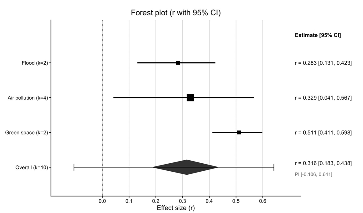
- Heterogeneity was assessed using Cochran’s Q statistic and the I² statistic. Forest plots were generated to visualize the overall and domain-specific pooled effect-size estimates. Publication bias was evaluated using funnel plots, Egger’s regression test (Egger et al., 1997), and the trim-and-fill method (Duval & Tweedie, 2000).
- All meta-analyses were conducted using R statistical software.
- GIS-Based Spatial Analysis
- An exploratory GIS-based spatial analysis was conducted using 426 administrative dongs in Seoul as the area-level units of analysis. The datasets included administrative boundary shapefiles, environmental facility location data, publicly supported housing records, and neighborhood-level household statistics. Potential environmental burden was operationalized using an environmental facility proximity indicator. A 300-meter buffer was generated around each environmental facility, and the proportion of buffer area within each administrative neighborhood was calculated. The 300-meter threshold was selected to ensure consistency and comparability across neighborhoods. The 300-m buffer was not intended to represent a universal physical boundary of environmental exposure or health risk. Rather, it was adopted as an operational proximity threshold for standardized neighborhood-level screening. Proximity-based indicators have been used in environmental justice screening approaches as proxies for potential environmental burden when direct exposure measurements are unavailable (Sadd et al., 2011). Accordingly, the indicator used here represents environmental facility proximity rather than measured environmental exposure. This indicator was designed to capture the proportion of each administrative dong located within the designated proximity zones surrounding environmental infrastructure facilities, rather than merely counting the number of facilities present. To avoid double counting, overlapping buffers were merged before spatial analysis. Buffer polygons were then intersected with neighborhood boundaries, and the total buffer area within each neighborhood was calculated. The environmental facility proximity indicator was subsequently derived by dividing the buffer area by the total area of the neighborhood. As a sensitivity check, the same procedure was repeated using a 500-m proximity threshold to examine whether the direction of the association and the spatial autocorrelation pattern were robust to an alternative buffer specification. Socioeconomic vulnerability was operationalized using the proportion of publicly supported housing. This measure was defined as the percentage of households residing in national housing and permanent rental housing relative to the total number of households within each neighborhood. The indicator was selected because it provides a comparable measure of housing vulnerability and residential constraints at the neighborhood level. Public housing records were geocoded and converted into spatial point data before being joined with neighborhood polygons. The number of national housing and permanent rental housing units was aggregated for each neighborhood and divided by the total number of households to calculate the publicly supported housing ratio. The association between the two indicators was explored using descriptive statistics, Pearson correlation analysis, and a simple bivariate regression. The regression was used only as a descriptive summary of the linear association and was not intended as a causal or spatially adjusted explanatory model.
- Zero values were treated as valid observations rather than missing data because neighborhoods without environmental facility buffers or publicly supported housing units remain important components of Seoul’s urban structure. Spatial clustering of environmental facility proximity was assessed using Global Moran’s I and Local Indicators of Spatial Association (LISA), which are commonly used to examine global and local patterns of spatial autocorrelation (Anselin, 1995). Spatial weights were constructed using a first-order Queen contiguity matrix, and statistical significance was evaluated through 999 permutations. LISA analysis was used to identify High–High, Low–Low, High–Low, and Low–High clusters. These analyses allowed the spatial distribution and clustering patterns of environmental facility proximity to be examined across Seoul. Spatial data processing and analysis were conducted using QGIS and GeoDa. GeoDa was used to support exploratory spatial data analysis and the assessment of global and local spatial autocorrelation (Anselin et al., 2006).
2. Materials and Methods
- Study Selection and Characteristics
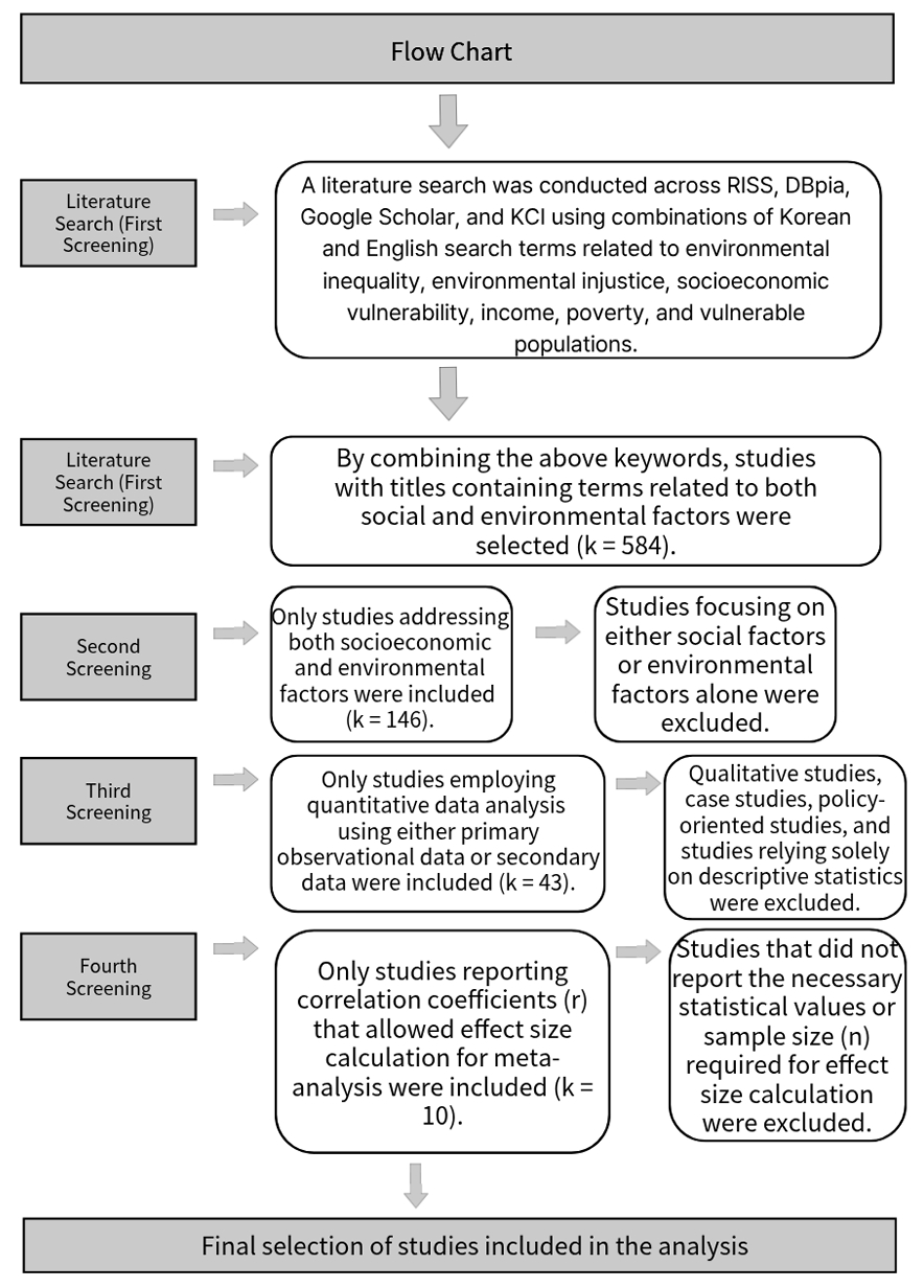
- Using the study-selection process organized with reference to the PRISMA framework, 584 records were initially identified through database searches and title screening.
- After reviewing abstracts and introductions, 146 studies addressing both environmental and socioeconomic factors were retained. Among these, 43 studies employed quantitative approaches to examine the relationship between the two variables. Ultimately, 10 studies reporting correlation coefficients or sufficient statistical information for effect-size calculation were included in the meta-analysis (Figure 1).
- The selected studies consisted of empirical investigations examining the relationship between environmental inequality and socioeconomic vulnerability. Although the studies differed in geographic context, spatial scale, environmental indicators, and socioeconomic measures, they shared the common objective of statistically assessing associations between environmental conditions and socioeconomic characteristics.
- The included studies covered multiple environmental domains: flood vulnerability (Park & Song, 2014; Seo & Han, 2019), air pollution and social deprivation (Chakraborty & Basu, 2021; Padilla et al., 2014; Verbeek, 2019; Næss et al., 2007), green-space accessibility (Myeong, 2017; Seo & Jun, 2011), toxicant exposure (Tyrrell et al., 2013), and transportation accessibility (Han et al., 2014). Socioeconomic indicators included income level, poverty measures, deprivation indices, and regional inequality indicators. Among the included studies, four focused on air pollution, two on green-space accessibility, two on flood risk, one on hazardous substance accumulation, and one on transportation accessibility (Table 1).
- Meta-Analysis Findings
- A random-effects meta-analysis of the 10 included effect sizes yielded a pooled correlation coefficient of r = 0.316 (95% CI: 0.183–0.438) (Table 2, Figure 2). The pooled estimate indicates that, on average, higher socioeconomic vulnerability was associated with more environmentally disadvantaged conditions across the included studies. However, this estimate represents an average association across heterogeneous research contexts and should not be interpreted as a universal magnitude of environmental inequality.
- Substantial heterogeneity was observed among the studies. Cochran’s Q statistic was 206.36 (df = 9, p < 0.001), and the I² value reached 95.64%, indicating that the variability among effect sizes could not be explained solely by sampling error (Table 3). Differences in environmental indicators, geographic settings, socioeconomic measures, and spatial units may have contributed to this heterogeneity. Therefore, the pooled effect size should be interpreted as an average association observed across diverse research contexts rather than a universal effect. The high heterogeneity is substantively informative as well as methodologically limiting, suggesting that the strength of environmental inequality is context-dependent rather than uniform across environmental domains and geographic settings.
- Subgroup analyses revealed variation across environmental domains. The two studies examining green-space accessibility yielded a pooled correlation coefficient of r = 0.511 (95% CI: 0.411–0.598), with no observed heterogeneity (I² = 0.00%). However, because this subgroup contained only two studies, the apparent absence of heterogeneity should be interpreted cautiously. Air pollution studies yielded a pooled correlation of r = 0.329 (95% CI: 0.041–0.567), although heterogeneity remained high (I² = 96.29%). Flood-related studies reported a pooled correlation of r = 0.283 (95% CI: 0.131–0.423) with moderate heterogeneity (I² = 41.32%) (Table 2, Table 3, Figure 2).
- Overall, the subgroup results suggest that the association between socioeconomic vulnerability and environmental disadvantage may vary across environmental domains. However, the small number of studies in several subgroups limits the precision of these estimates and the strength of comparisons between domains. These findings should therefore be interpreted as exploratory rather than as definitive evidence that any particular environmental domain exhibits a stronger or more stable association.
- Publication Bias Assessment
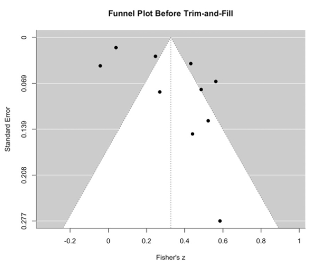
- To assess potential funnel plot asymmetry and small-study effects, a funnel plot was examined and Egger’s regression test was conducted (Figure 3). Egger’s test indicated statistically significant funnel plot asymmetry (t = 2.437, df = 8, p = 0.041), suggesting the possibility of small-study effects or publication bias. However, this finding should be interpreted cautiously given the small number of included studies and the substantial between-study heterogeneity.
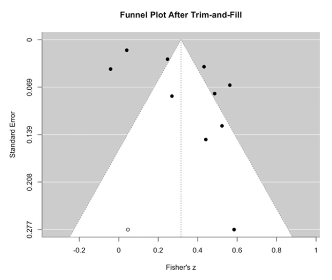
- A trim-and-fill analysis was subsequently conducted as a sensitivity analysis to examine the robustness of the pooled effect estimate (Figure 3, Figure 4). After adjustment, the pooled correlation coefficient was r = 0.305 (95% CI: 0.175–0.425), slightly lower than the original estimate of r = 0.316 (95% CI: 0.183–0.438). The adjusted confidence interval remained above zero, indicating that the positive average association persisted after adjustment. However, the adjusted 95% prediction interval ranged from −0.115 to 0.633, crossing zero and suggesting that the direction and magnitude of the association may vary across research settings.
- Overall, the trim-and-fill analysis yielded an adjusted pooled estimate that was broadly consistent with the original result. Nevertheless, the significant Egger’s test and the limited number of included studies warrant caution in interpreting the possibility of publication bias. These diagnostics should therefore be regarded as exploratory evidence of potential small-study effects rather than definitive evidence of publication bias.
- GIS-Based Spatial Analysis
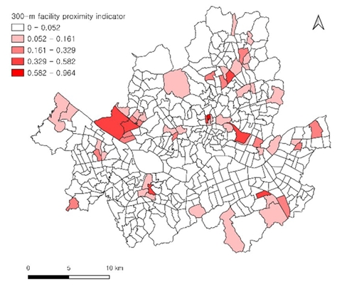
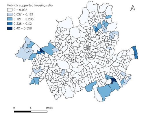
- An exploratory GIS-based spatial analysis was conducted across 426 administrative dongs in Seoul. The distributions of both the 300-m environmental facility proximity indicator and the publicly supported housing ratio exhibited a strong concentration around zero or relatively low values. The median values of both indicators were close to zero, while relatively high values were observed in a limited number of administrative dongs for each indicator. These distributional patterns indicate that the two indicators were spatially uneven, but they do not by themselves demonstrate direct overlap between high environmental facility proximity and high housing vulnerability (Figure 5, Figure 6).
- Pearson correlation analysis between the 300-m environmental facility proximity indicator and the publicly supported housing ratio yielded a weak positive association (r = 0.187). A descriptive bivariate regression produced an R² value of 0.035, indicating that publicly supported housing alone explained only a limited portion of the spatial variation in environmental facility proximity. This regression is interpreted descriptively rather than as a spatially adjusted explanatory model.
- As a sensitivity check, the 500-m proximity indicator showed a similar weak positive association with the publicly supported housing ratio (r = 0.195, R² = 0.038), suggesting that the direction of the association was not solely dependent on the 300-m threshold. Nevertheless, the explanatory power remained limited under both buffer specifications. Therefore, a more comprehensive understanding of the spatial distribution of environmental facility proximity requires consideration of additional socioeconomic and urbanspatial factors, including land use, urban planning, facility siting, demographic composition, income, aging populations, green space accessibility, flood risk, and air quality.
- Spatial Clustering of Environmental Facility Proximity
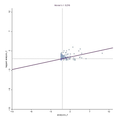
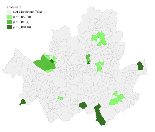
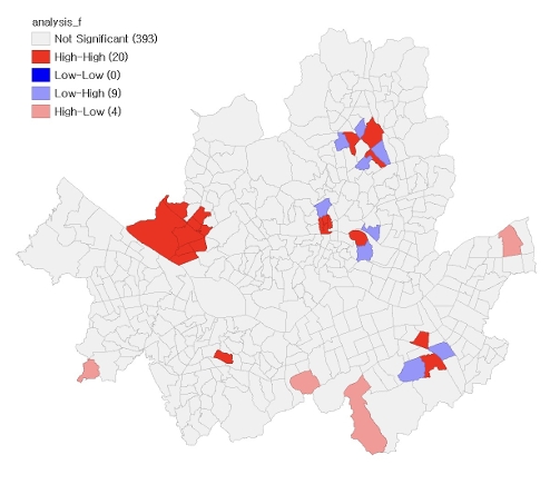
- To examine the spatial clustering of the environmental facility proximity indicator, measured as the proportion of land area within a 300-m proximity zone surrounding environmental infrastructure facilities, a Global Moran’s I analysis was conducted. The Global Moran’s I analysis produced statistically significant positive spatial autocorrelation for the 300-m environmental facility proximity indicator (I = 0.216, z = 7.790, pseudo p = 0.001; 999 permutations) (Figure 7). This finding suggests that the environmental facility proximity indicator was spatially clustered rather than randomly distributed across Seoul, with neighboring administrative dongs tending to exhibit similar levels of facility proximity. The 500-m sensitivity analysis also showed statistically significant positive spatial autocorrelation (I = 0.309, z = 11.195, pseudo p = 0.001), indicating that the spatial clustering pattern was robust to the alternative proximity threshold. Local Indicators of Spatial Association (LISA) analysis further identified statistically significant local spatial association in 33 of the 426 administrative dongs: 20 at p ≤ 0.05, 7 at p ≤ 0.01, and 6 at p ≤ 0.001 (Figure 8). Figure 8 indicates where the local spatial association was statistically significant, whereas Figure 9 classifies the significant local patterns into cluster and spatial-outlier categories. The LISA cluster map showed 20 High–High clusters, 9 Low–High outliers, and 4 High–Low outliers, with no Low–Low clusters (Figure 9). In Figure 9, High–High indicates administrative dongs with high environmental facility proximity values surrounded by neighboring dongs with similarly high values, whereas Low–Low indicates low-value dongs surrounded by low-value neighboring dongs. Low–High and High–Low represent spatial outliers: Low–High indicates low-value dongs surrounded by high-value neighboring dongs, while High–Low indicates high-value dongs surrounded by low-value neighboring dongs (Figure 9). These results indicate localized concentrations of high environmental facility proximity and local spatial outliers, rather than direct evidence of spatial overlap between environmental burden and housing vulnerability.
3. Results
- Interpretation of Main Findings
- This study examined environmental inequality through two complementary analytical components: a systematic review and meta-analysis of previous empirical evidence and an exploratory area-level GIS analysis of Seoul. The meta-analysis identified a positive pooled association on average (Table 2, Figure 2), whereas the Seoul analysis showed a weaker positive area-level association between environmental facility proximity and publicly supported housing, together with localized spatial clustering of the proximity indicator (Figure 7, Figure 8, Figure 9). These findings should not be interpreted as direct replication across analytical levels; rather, they provide complementary evidence regarding general cross-study tendencies and place-specific spatial patterns.
- The pooled effect size suggests an average tendency for environmentally disadvantaged conditions to be positively associated with socioeconomic vulnerability across the included studies.
- These findings are consistent with the environmental justice perspective, which argues that environmental risks and environmental benefits may be distributed unevenly according to socioeconomic conditions. As the present meta-analysis represents a quantitative synthesis based on correlation coefficients, its primary objective is to determine whether the relationship between environmental inequality and socioeconomic vulnerability is repeatedly observed across diverse research contexts.
- Overall heterogeneity across the meta-analysis was very high (I² = 95.64%), indicating that differences in effect sizes among the included studies cannot be explained solely by sampling error (Table 3). Variations in environmental indicators, geographical contexts, socioeconomic measures, and spatial units are likely to contribute to this variability. Importantly, the heterogeneity is not only a methodological limitation but also substantively informative, because it suggests that the magnitude of environmental inequality may be strongly context-, indicator-, and scale-dependent. The two green-space studies yielded relatively large and similar correlation estimates, but the very small subgroup size precludes strong conclusions regarding consistency. Likewise, positive pooled estimates in the air-pollution and flood subgroups should be interpreted cautiously because of the limited number of studies and remaining heterogeneity. The subgroup findings therefore serve primarily as exploratory indications of possible domain-specific variation.
- In the environmental-domain subgroup analysis, the pooled correlation for green-space accessibility was numerically larger than those for air pollution and flood risk (Table 2, Figure 2). However, the small number of studies in each subgroup prevents firm conclusions about differences in effect sizes across environmental domains. Moreover, whereas the meta-analysis encompassed both environmental burdens and environmental benefits, the Seoul GIS analysis relied on a narrower set of proxy indicators: proximity to environmental infrastructure facilities and the proportion of publicly supported housing. This difference in measurement scope may help explain why the strengths of the observed associations differed between the two analyses, but its contribution was not directly tested in this study. In addition, the meta-analysis synthesized studies conducted across different geographic settings and spatial units, using varied socioeconomic indicators, whereas the Seoul GIS analysis focused on a single city at the administrative-dong level and used publicly supported housing as a proxy for housing vulnerability. These differences in geographic context, spatial scale, and indicator selection further limit direct comparisons of the correlation magnitudes. Their individual contributions to the observed difference were not separately assessed. Accordingly, the Seoul GIS findings should be interpreted as complementary, place-specific evidence of associations and spatial patterns rather than as confirmation or strengthening of the meta-analytic findings.
- The GIS analysis of Seoul revealed a weak positive area-level association between the 300-m environmental facility proximity indicator and the publicly supported housing ratio. This result should not be interpreted as direct evidence that high environmental burden and high housing vulnerability spatially overlap in specific neighborhoods. Rather, it indicates that, at the administrative-dong level, areas with higher environmental facility proximity tended to show somewhat higher publicly supported housing ratios. The coefficient of determination (R² = 0.035) indicates that publicly supported housing alone explains only a limited portion of the spatial variation in environmental facility proximity. The 500-m sensitivity analysis produced a similar weak positive association and statistically significant spatial autocorrelation, suggesting that the observed direction and clustering pattern were not solely artifacts of the 300-m buffer specification. However, the explanatory power remained limited, and the results should not be interpreted as evidence of direct spatial overlap between high environmental burden and high housing vulnerability. Therefore, a more comprehensive understanding of the spatial distribution of environmental facility proximity requires consideration of additional social and environmental indicators, including income, aging populations, recipients of basic livelihood security benefits, single-person households, flood risk, green space accessibility, and air quality.
- The spatial autocorrelation analysis demonstrated that the environmental facility proximity indicator was not randomly distributed across Seoul but tended to cluster among neighboring administrative dongs with similar levels of facility proximity (Figure 7). The LISA analysis identified 20 High–High clusters, indicating localized concentrations where high values of the proximity indicator were surrounded by neighboring administrative dongs with similarly high values (Figure 9). The analysis also identified 9 Low–High outliers and 4 High–Low outliers, suggesting local deviations from surrounding spatial patterns (Figure 9). These findings indicate localized spatial clustering of facility proximity and may help identify candidate areas for further environmental and socioeconomic investigation. However, because the LISA analysis was conducted on the environmental facility proximity indicator, the results should not be interpreted as direct evidence that environmental burden and housing vulnerability are spatially clustered together.
- Policy Relevance and Screening Implications for Urban Environmental Governance
- Given the exploratory nature of the Seoul analysis and the weak bivariate association observed between the two proxy indicators, the GIS findings should not be used as a stand-alone basis for designating environmentally unjust neighborhoods or determining direct policy intervention. Rather, the framework is more appropriately interpreted as a first-stage spatial screening approach for identifying candidate areas that may warrant more detailed environmental and socioeconomic assessment. Environmental justice screening approaches similarly emphasize the use of environmental and social vulnerability indicators to identify areas for subsequent investigation rather than to establish definitive causal conclusions (Sadd et al., 2011). In this sense, the policy relevance of the present framework lies in a staged process of screening, validation, and intervention.
- Although this study does not directly evaluate ESG performance, its screening framework is relevant to ESG-informed urban environmental governance in a limited sense. The environmental facility proximity indicator corresponds to the environmental dimension of ESG, as it reflects the spatial distribution of potential environmental burdens, while the publicly supported housing ratio captures one aspect of the social dimension, namely the residential constraints of potentially vulnerable households. The staged process of screening, validation, and intervention proposed above relates to the governance dimension, in that it offers a transparent and reproducible basis for prioritizing areas for further assessment and for documenting how such priorities are set. For instance, public agencies responsible for environmental infrastructure or public housing could use such screening results as one input when reviewing environmental and social risks around vulnerable residential areas. Nevertheless, these connections are conceptual rather than empirical: the present study does not construct ESG indicators, assess the ESG performance of any organization, or evaluate governance outcomes.
- Areas identified through initial screening should undergo further validation before specific policy measures are considered. Such validation may incorporate direct environmental measurements, additional socioeconomic indicators, field investigation, resident consultation, and other locally relevant information. Depending on the environmental conditions subsequently confirmed, measures such as environmental monitoring, information provision, resident participation, or locally appropriate environmental improvements may be considered. However, the present analysis does not provide sufficient evidence to determine which specific interventions would be appropriate for individual neighborhoods.
- The numerical findings observed in Seoul are not intended to be statistically generalized to other cities. Rather, the potentially transferable contribution lies in the analytical framework, which may be adapted and tested in other urban contexts using locally appropriate environmental and socioeconomic indicators.
- For policy applications, spatial analysis results should be combined with field investigations, resident consultations, additional environmental datasets, and social vulnerability indicators. Such an approach can reveal inequalities concealed by district- or city-level averages and provide foundational evidence for the development of Korean environmental justice indicators and urban environmental governance indicators in the future.
- Limitations
- This study combined meta-analysis and GIS spatial analysis to examine the relationship between environmental inequality and socioeconomic vulnerability. Nevertheless, several limitations should be acknowledged.
- First, the number of studies included in the meta-analysis was limited to ten. This was primarily due to the insufficient accumulation of prior studies that quantitatively examined the relationship between environmental inequality and socioeconomic vulnerability and reported the statistical information necessary for effect size estimation. Consequently, the pooled effect size should be regarded as an exploratory summary estimate derived from a limited body of evidence rather than as a definitive population-level effect, and it should be reevaluated as additional eligible studies become available.
- Second, substantial heterogeneity was observed across the meta-analysis. To account for between-study variation, this study employed a random-effects model and conducted subgroup analyses by environmental category. However, the included studies differed considerably in terms of environmental indicators, socioeconomic indicators, spatial units, and geographical contexts, limiting the ability to disentangle the specific sources of effect size variation. The high heterogeneity also limits the extent to which the pooled estimate can be generalized to any specific environmental domain, city, or population.
- Third, the possibility of publication bias or small-study effects was identified. The funnel plot showed asymmetry (Figure 3), Egger’s regression test indicated statistically significant asymmetry, and the trim-and-fill analysis imputed one potentially missing study (Figure 4). Although the direction and statistical significance of the overall effect remained stable after adjustment, the relatively small number of included studies limits the robustness of publication bias assessments. To address this concern, both adjusted and unadjusted effect sizes were reported in the present study.
- Fourth, although spatial autocorrelation was identified in the environmental facility proximity indicator, the present study did not estimate spatial regression models such as spatial lag or spatial error models. The simple regression was used as a descriptive extension of the bivariate analysis rather than as a causal or spatially adjusted explanatory model. Consequently, the regression estimates may be affected by unmodeled spatial dependence and should be interpreted cautiously. Future confirmatory research should employ spatial regression models to determine whether the observed association persists after spatial dependence is explicitly accounted for.
- Fifth, the scope of environmental and social vulnerability indicators included in the GIS analysis was limited. This study used the proportion of land area within a 300-meter buffer of environmental infrastructure facilities as a proxy measure of potential environmental burden and the proportion of publicly supported housing as a proxy measure of housing vulnerability. Although proximity to environmental infrastructure facilities is useful for assessing spatial overlap between facilities and residential areas at the administrative-dong level, it does not fully capture the diverse environmental burdens present in urban settings, including air pollution, odor, noise, traffic exposure, thermal stress, green space accessibility, and flood risk. Likewise, the proportion of publicly supported housing reflects only one aspect of housing vulnerability and does not encompass broader dimensions of socioeconomic vulnerability, such as income, poverty, assets, employment status, and health conditions.
- Sixth, the 300-m proximity measure should be regarded as one operational representation of local facility proximity rather than as a definitive spatial extent of environmental exposure or health risk. Although this study conducted a 500-m sensitivity analysis, additional thresholds such as 100 m and 1 km were not examined. Therefore, the robustness of the observed patterns across a wider range of distance specifications should be further assessed in future research.
- Seventh, the use of administrative dongs as the primary unit of analysis may not adequately capture micro-level spatial variations within neighborhoods. Even within the same administrative dong, residents’ levels of environmental exposure may differ depending on residential location, actual distance from facilities, population density, land-use characteristics, and neighborhood boundaries. Future research could utilize grid-based datasets, building-level data, and population-weighted exposure indicators to investigate intra-neighborhood spatial disparities in greater detail.
- Conclusion
- This study examined the relationship between environmental inequality and socioeconomic vulnerability by integrating a systematic literature review, meta-analysis, and GIS spatial analysis at the administrative-dong level in Seoul. The significance of this study lies in its simultaneous examination of quantitative patterns reported in previous studies and the detailed spatial distributions observed in an actual urban environment. In doing so, the study extended the discussion of environmental inequality beyond individual cases or single indicators by linking synthesized evidence from the literature with spatial disparities within the city.
- The meta-analysis revealed an overall positive association between environmental inequality and socioeconomic vulnerability. Although substantial heterogeneity was observed across the included studies, this finding suggests that the manifestation of environmental inequality may vary according to environmental characteristics, regional contexts, socioeconomic indicators, and spatial scales. Therefore, the pooled effect size reported in this study should be interpreted as a summary estimate representing the average association repeatedly observed across diverse research settings.
- The GIS analysis of Seoul identified a weak positive area-level association between the 300-m environmental facility proximity indicator and the publicly supported housing ratio. In addition, the environmental facility proximity indicator exhibited localized spatial clustering in certain areas. The 500-m sensitivity analysis produced similar directional results, suggesting that the weak positive association and spatial clustering pattern were not solely dependent on the 300-m proximity threshold. These findings suggest that administrative-dong-level spatial screening can help identify candidate areas for further environmental and socioeconomic investigation. However, because this study did not directly analyze the spatial overlap of high environmental burden and high housing vulnerability, the results should not be interpreted as definitive evidence of environmental injustice or as a direct basis for policy intervention.
- These findings may also be considered in relation to broader urban and community development agendas, including SDG 10 and SDG 11, as well as ESG-informed governance practices that incorporate environmental and social vulnerability considerations. However, this study does not evaluate progress toward these goals or assess the outcomes of specific policy interventions. Rather, by showing how environmental facility proximity and a proxy indicator of housing vulnerability can be examined at the administrative-dong level, the study illustrates how spatial screening may provide preliminary evidence for identifying intra-urban disparities. Accordingly, the SDG and ESG relevance of this study should be understood as indirect and screening-oriented, rather than as evidence that specific SDG targets have been achieved or that particular areas require immediate policy intervention.
- Future research should incorporate a broader range of environmental indicators, including air pollution, noise, odor, thermal environments, green space accessibility, and flood risk, together with direct socioeconomic measures such as income, poverty, aging populations, health conditions, and housing instability. Moreover, integrating longitudinal datasets, resident complaint records, and health-related data would enable a more comprehensive examination of how spatial relationships between environmental burdens and social vulnerability evolve over time and whether policy interventions contribute to reducing regional disparities. As data continue to accumulate, administrative-dong-level spatial analysis can be repeatedly applied and refined, serving as a foundational tool for the development of Korean environmental justice indicators and urban environmental governance frameworks.
4. Discussion and Conclusions
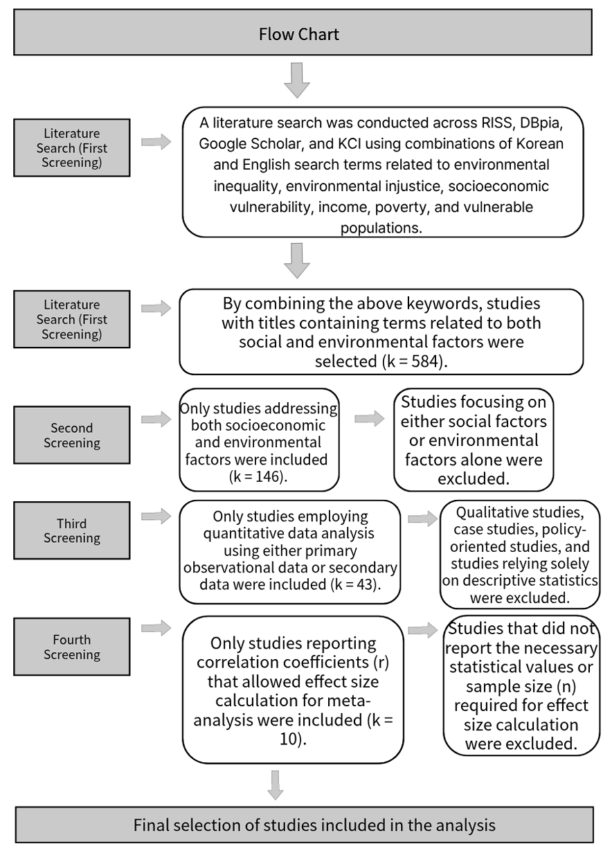
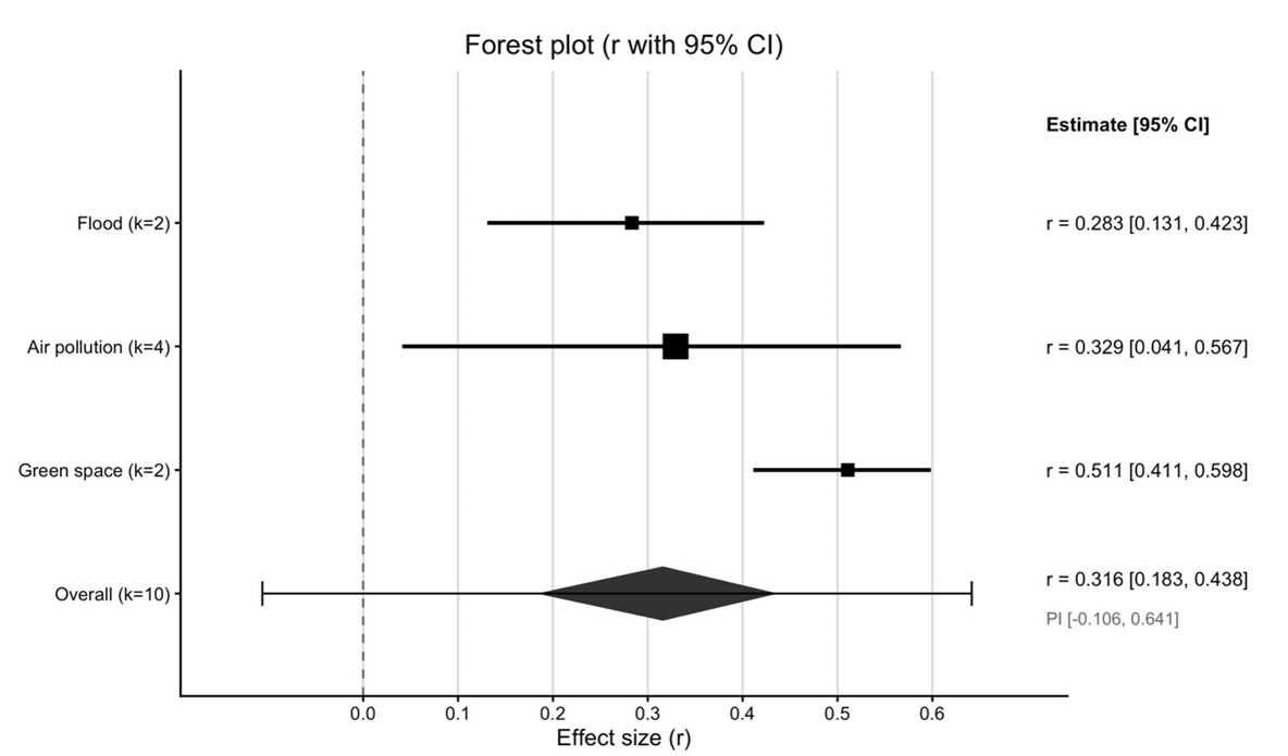
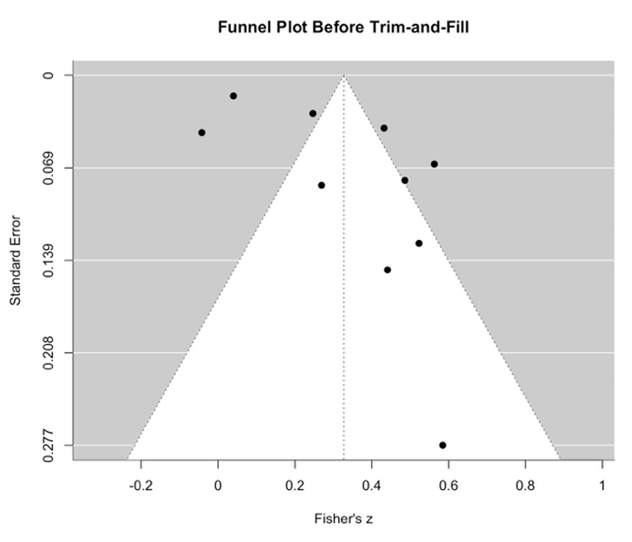
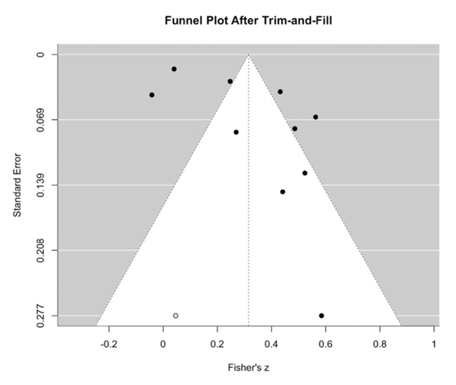
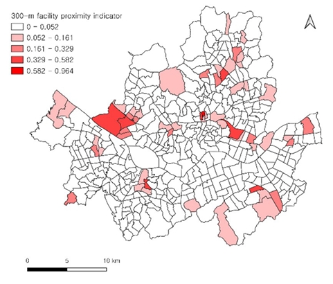
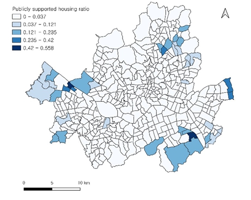
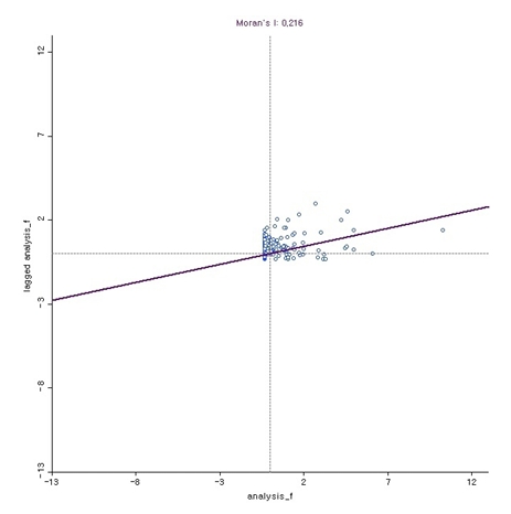
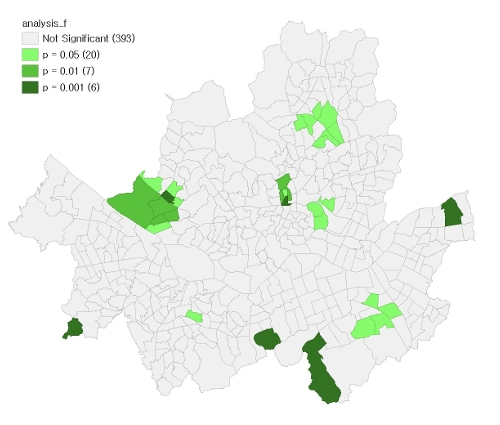
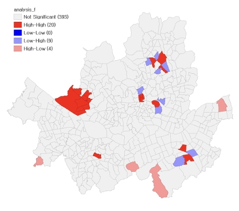
Table 1.Characteristics of Included Studies
| Authors (Year) | Study | Analytical Sample(n) | Socioeconomic Indicator | Environmental Indicator | Effect Size(r) |
|---|---|---|---|---|---|
| (Park & Song, 2014) | Empirical Study on Environmental Justice through Correlation Analysis of the Flood Vulnerability Indicator and the Ratio of the Poor Population. | n = 50 | Poverty Vulnerability Index (PVI) | Flood Vulnerability Indicator (FVI) | r = 0.41441 |
| (Chakraborty & Basu, 2021) | Air Quality and Environmental Injustice in India: Connecting Particulate Pollution to Social Disadvantages. | n = 640 | Scheduled Caste population | PM2.5 mean concentration (2010) | r = 0.407 |
| (Myeong, 2017) | Green Space Accessibility Analysis in Terms of Environmental Justice. | n = 229 | Percentage of single mother households | Lack of park and green space (reverse-coded) | r = 0.51 |
| (Padilla et al., 2014) | Air quality and social deprivation in four French metropolitan areas – A localized spatiotemporal environmental inequality analysis. | n = 545 | Deprivation index | NO2 concentration (annual mean) | r = -0.042 |
| (Tyrrell et al., 2013) | Associations between socioeconomic status and environmental toxicant concentrations in adults in the USA: NHANES 2001–2010. | n = 4196 | Poverty income ratio (PIR) | Blood lead concentration | r = 0.04 |
| (Verbeek, 2019) | Unequal residential exposure to air pollution and noise: A geospatial environmental justice analysis for Ghent, Belgium | n = 164 | income | Annual mean NO₂ concentration | r = 0.451 |
| (Han et al., 2014) | Correlation Analysis between Median Household Income and LEED-Certified Public Transportation Access | n = 150 | income | Public transportation access (light rail stations, LEED-qualified) | r = 0.263 |
| (Seo & Jun, 2011) | Environmental Equity Analysis of the Accessibility of Urban Neighborhood Parks in Daegu City | n = 16 | Basic Pension Recipient Rate | Lack of park and green space development area (reverse-coded) | r = 0.526 |
| (Seo & Han, 2019) | Exploring the Relationship Between Floods and Socially Vulnerable Groups: The Case of Jeju | n = 1230 | The elderly | Urban flooding | r = 0.242 |
| (Næss et al., 2007) | Air Pollution, Social Deprivation, and Mortality: A Multilevel Cohort Study. | n = 66 | Living in flat | PM2.5 | r = 0.48 |
Table 2.Pooled Correlation Coefficients by Study Group
Table 3.Heterogeneity Statistics
| Study group | k | Q | I²(%) |
|---|---|---|---|
| Total | 10 | 206.36 | 95.64 |
| Air pollution studies | 4 | 80.86 | 96.29 |
| Studies examining green-space accessibility | 2 | 0.006 | 0.00 |
| Flood-related studies | 2 | 1.70 | 41.32 |
- Anselin, L. (1995). Local indicators of spatial association—LISA. Geographical Analysis, 27(2), 93-115. https://doi.org/10.1111/j.1538-4632.1995.tb00338.xArticle
- Anselin, L., Syabri, I., & Kho, Y. (2006). GeoDa: An introduction to spatial data analysis. Geographical Analysis, 38(1), 5-22. https://doi.org/10.1111/j.0016-7363.2005.00671.xArticle
- Chakraborty, J., & Basu, P. (2021). Air quality and environmental injustice in India: Connecting particulate pollution to social disadvantages. In-ternational Journal of Environmental Research and Public Health, 18(1), Article 304. https://doi.org/10.3390/ijerph18010304ArticlePubMedPMC
- DerSimonian, R., & Laird, N. (1986). Meta-analysis in clinical trials. Controlled Clinical Trials, 7(3), 177-188. https://doi.org/10.1016/0197-2456(86)90046-2ArticlePubMedPMC
- Duval, S., & Tweedie, R. (2000). Trim and fill: A simple funnel-plot-based method of testing and adjusting for publication bias in meta-analysis. Biometrics, 56(2), 455-463. https://doi.org/10.1111/j.0006-341X.2000.00455.xArticlePubMedPMC
- Egger, M., Davey Smith, G., Schneider, M., & Minder, C. (1997). Bias in meta-analysis detected by a simple, graphical test. BMJ, 315(7109), 629-634. https://doi.org/10.1136/bmj.315.7109.629ArticlePubMedPMC
- Hajat, A., Hsia, C., & O’Neill, M. S. (2015). Socioeconomic disparities and air pollution exposure: A global review. Current Environmental Health Reports, 2(4), 440-450. https://doi.org/10.1007/s40572-015-0069-5ArticlePubMedPMC
- Han, H. S., Kim, B.-Y., Park, Y. J., & Son, K. (2014). Correlation analysis between median household income and LEED-certified public trans-portation access. Journal of the Korea Institute of Building Construction, 14(3), 266-272. https://doi.org/10.5345/JKIBC.2014.14.3.266Article
- Mohai, P., Pellow, D., & Roberts, J. T. (2009). Environmental justice. Annual Review of Environment and Resources, 34, 405-430. https://doi.org/10.1146/annurev-environ-082508-094348Article
- Myeong, S. (2017). Green space accessibility analysis in terms of environmental justice. Korea Environment Institute. https://doi.org/10.23000/TRKO201800014411
- Næss, Ø., Piro, F. N., Nafstad, P., Davey Smith, G., & Leyland, A. H. (2007). Air pollution, social deprivation, and mortality: A multilevel cohort study. Epidemiology, 18(6), 686-694. https://doi.org/10.1097/EDE.0b013e3181567d14ArticlePubMed
- Padilla, C. M., Kihal-Talantikite, W., Vieira, V. M., Rossello, P., Le Nir, G., Zmirou-Navier, D., & Deguen, S. (2014). Air quality and social deprivation in four French metropolitan areas—A localized spatio-temporal environmental inequality analysis. Environmental Research, 134, 315-324. https://doi.org/10.1016/j.envres.2014.07.017ArticlePubMedPMC
- Page, M. J., McKenzie, J. E., Bossuyt, P. M., Boutron, I., Hoffmann, T. C., Mulrow, C. D., Shamseer, L., Tetzlaff, J. M., Akl, E. A., Brennan, S. E., Chou, R., Glanville, J., Grimshaw, J. M., Hróbjartsson, A., Lalu, M. M., Li, T., Loder, E. W., Mayo-Wilson, E., McDonald, S., & Moher, D. (2021). The PRISMA 2020 statement: An updated guideline for reporting systematic reviews. BMJ, 372, Article n71. https://doi.org/10.1136/bmj.n71ArticlePubMedPMC
- Park, H. N., & Song, J. M. (2014). Empirical study on environmental justice through correlation analysis of the flood vulnerability indicator and the ratio of the poor population. Journal of Korea Planning Association, 49(7), 169-186. https://doi.org/10.17208/jkpa.2014.11.49.7.169Article
- Sadd, J. L., Pastor, M., Morello-Frosch, R., Scoggins, J., & Jesdale, B. (2011). Playing it safe: Assessing cumulative impact and social vulnerability through an environmental justice screening method in the South Coast Air Basin, California. International Journal of Environmental Research and Public Health, 8(5), 1441-1459. https://doi.org/10.3390/ijerph8051441ArticlePubMedPMC
- Schlosberg, D. (2007). Defining environmental justice: Theories, movements, and nature. Oxford University Press. https://doi.org/10.1093/acprof:oso/9780199286294.001.0001
- Seo, H. J., & Jun, B. W. (2011). Environmental equity analysis of the accessibility of urban neighborhood parks in Daegu City. Journal of the Ko-rean Association of Geographic Information Studies, 14(4), 221-237.Article
- Seo, J., & Han, W. (2019). Exploring the relationship between floods and socially vulnerable groups: The case of Jeju. Journal of the Korean Society of Hazard Mitigation, 19(4), 103-113. https://doi.org/10.9798/KOSHAM.2019.19.4.103Article
- Tyrrell, J., Melzer, D., Henley, W., Galloway, T. S., & Osborne, N. J. (2013). Associations between socioeconomic status and environmental toxicant concentrations in adults in the USA: NHANES 2001–2010. Environment International, 59, 328-335. https://doi.org/10.1016/j.envint.2013.06.017ArticlePubMed
- Verbeek, T. (2019). Unequal residential exposure to air pollution and noise: A geospatial environmental justice analysis for Ghent, Belgium. SSM - Population Health, 7, Article 100340. https://doi.org/10.1016/j.ssmph.2018.100340ArticlePubMedPMC
- Wolch, J. R., Byrne, J., & Newell, J. P. (2014). Urban green space, public health, and environmental justice: The challenge of making cities “just green enough.”. Landscape and Urban Planning, 125, 234-244. https://doi.org/10.1016/j.landurbplan.2014.01.017Article
References
Figure & Data
References
Citations
Citations to this article as recorded by 
 PubReader
 ePub Link
 Cite
 XML Download